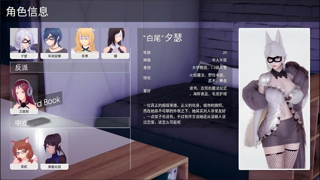
Ana səhifə

Supplementary information of Watching Two Conjugated Polymer Chains Breaking Each Other When Colliding in Solution


Yüklə 1.62 Mb.
tarix27.06.2016
ölçüsü1.62 Mb.
Supplementary information of

Watching Two Conjugated Polymer Chains Breaking Each Other When Colliding in Solution

Yuxi Tian,1 Marina V. Kuzimenkova1, Mingyi Xie1, Matthias Meyer1, Per-Olof Larsson2 and Ivan G. Scheblykin1,*

1Chemical Physics, Lund University, Box 124, SE-22100, Lund, Sweden

2Pure and Applied Biochemistry, Lund University, Box 124, SE-22100, Lund, Sweden

* Email: Ivan.Scheblykin@chemphys.lu.se


Table of contents

  1. Snapshots and a movie of two MEH-PPV molecules colliding with each other

  2. Total fluorescence intensity during the reaction

  3. Snapshots and a movie of the chain rupture of a single MEH-PPV chain

  4. Only Brownian motion is present

  5. Estimation of the chance for two polymer chains to split at the same time

  6. Probability of one-chain rupture

  7. Estimation of the chain scission quantum yield

  8. Effect of oxygen

  9. Estimation of the polymer coil size of MEH-PPV

  10. Estimation of the diffusion coefficient of MEH-PPV

  11. Estimation of the chain relaxation time and the excitation rate at the contact point

  12. Estimation of physical collision probability by Monte-Carlo simulation

1. Snapshots and a movie of two MEH-PPV molecules colliding with each other


Figure S1. Sequential snapshots following two diffusing MEH-PPV chains, which collide with each other and split into four chains.

Movie 1 Collision process of two MEH-PPV chains showing simultaneous rupture. The time scale for the video was slowed down by half (10 fps).

2. Total fluorescence intensity during the reaction


Figure S2 Average fluorescence intensity in the region of interest during the chain collision shown in Fig.1. Inserts show collision. The frame before the bright spots came into the field of view was used to calculate the background signal which was subtracted.

Total fluorescence intensity over the region of interest (ROI) was analyzed during the collision process (Fig. S2). The total intensity of the reactants (two chains) is approximately equal to the intensity of the products (four chains). Fluctuations are due to the inhomogeneous excitation density. These results strongly support the hypothesis that the daughter fragments originate from their parent molecules.


3. Snapshots and a movie of the chain rupture of a single MEH-PPV chain


Figure S3. Snapshots showing self-splitting of a single MEH-PPV chain.

Movie 2 Self-splitting of a single MEH-PPV polymer chain. The time scale for the video was slowed down by half (10 fps).

4. Only Brownian motion is present

As shown in Fig. 1c in the main text, the solution stays in between two glass cover slips. The measurements were done about half an hour after the sample preparation to let the solution become stable to avoid any flow. Even though the evaporation of the solvent from the edge of the cover slips (10 mm away from the observation point) could induce a tiny flow, the flow rate at the observation point (centre of the sample) would be negligible. Another factor which can possibly induce flow in the system is the laser irradiation. However, only MEH-PPV molecules in the system can absorb the excitation light and produce some heat. All other components such as solvent, glass and the PMMA matrix would contribute negligibly to the light absorption. Considering the extremely low concentration of the MEH-PPV molecules, we would not expect any laser-heating-induced flow. Most importantly, SMS allowed us to directly look at the diffusion of individual molecules and observe random diffusion of the polymer chains as shown in Fig. S4. Based on these arguments, we conclude that there is no appreciable shear force induced by liquid flow in our sample system and the collision must be caused by Brownian motion only.

5. Estimation of the chance for two polymer chains to split at the same time

From experiments we got the kinetics of the chain rupture as shown in Fig. 2b. The curve was fitted by a single exponential decay:


 with τ = 0.7 s.

Where t is the time before splitting and  is characteristic lifetime time of individual polymer chains.


For an exponential process, the rate constant of the chain rupture is  and the probability of the chain rupture is:


In our experiments, the exposure time of each frame is 50 ms, i.e.  and thus the probability of a polymer chain rupture in one frame is:


For two molecules to split simultaneously in one frame the probability is:


.

6. Probability of one-chain rupture

About 13±2% of the visual-collision events generated three fragments, which shows that only one of the parent chains was split. As calculated in section 5, the probability of independent chain rupture within one frame is 7%. Since there are two chains in the same spot for each visual-collision event, the probability of one-chain rupture should be twice as high, i.e. 14%, which agrees very well with our observation of 13%. Such close agreement strongly suggests that one-chain ruptures observed in visual collisions happen mostly without involvement of the second chain.

7. Estimation of the chain scission quantum yield

The excitation rate (R) of the whole polymer (N monomers) can be calculated based on the absorption cross section per monomer (σ), the excitation wavelength (λ) and excitation power (P):


Where  - the Plank constant and с - speed of light. Under our experimental conditions (N=3100; P=10 W/cm2; λ=458 nm; σ=4.19×10⁻¹⁷ cm2), the excitation rate was estimated to be 3×10⁶ s-1.

Each polymer chain can be excited for 2×10⁶ times before splitting (within 0.7 s). The splitting quantum yield is thus 510-7.

So, with excitation power in the order of 0.001 W/cm2 (1% of sunlight power, close to room-light conditions) the Mn of such long chains (800 kDa) should decrease by 1/2 after about 0.7 s * (10 W/cm2)/(0.001 W/cm2) = 7000 s ≈ 2 hours.


8. Effect of oxygen

To investigate the effect of oxygen in the chain splitting events, an extra experiment was carried out in an oxygen-free atmosphere. By preparing the sample in a glove box and sealing the sample in a N2-filled sample chamber during the measurement, we tried our best to reduce the oxygen concentration as much as possible. As shown by Movie 3, under this condition, the self-splitting process is significantly suppressed.


Movie 3. A single MEH-PPV polymer chain diffuses in the excitation area over 20 seconds and leaves without chain splitting. The time scale for the video was slowed down by half (10 fps). Compare this with Movie 2 showing the sample prepared at the ambient conditions.

9. Estimation of the polymer coil size of MEH-PPV

As reported, the Kuhn length (b) of MEH-PPV varies from 12 to 65 nm depending on the chemical defects and the measurement methods3. Here we use the value of 13 nm for MEH-PPV in toluene4, which corresponds to about 20 monomers. For our sample, the molecular weight is about 800 kDa which means 155 Kuhn segments. This value is an underestimation, because in the measurement we are biased to observe the largest molecules due to their higher brightness and slower diffusion.

The solvent toluene was considered as a theta solvent for MEH-PPV. For simplicity, we assume the molecules as spheres and the radius (R) can be thus calculated5 as:


10. Estimation of the diffusion coefficient of MEH-PPV

Seventy individual molecules were tracked during 20 frames (1 s) and their final positions noted, See Fig. S4.


Figure S4 Relative position of 70 individual polymer chains after 20 frames (1 s). Initial position was shifted to (0,0) for each molecule.

The diffusion coefficient can be calculated:


The value is quite close to the theoretically calculated value, based on the Stokes-Einstein equation for diffusion, using 554 µPaS as viscosity value for toluene6.


kB = Boltzmann’s constant, T = absolute temperature, η= viscosity, R = molecule radius.


11. Estimation of the chain relaxation time and the excitation rate at the contact point

The chain relaxation time is of the order of time needed for the chain to diffuse over the distance equal to the polymer coil radius (ca. 100 nm). With the measured diffusion coefficient of 7.7 µm2/s as estimated above, we would estimate the chain relaxation time:


As calculated in Section 7, the excitation rate of the whole polymer is 3×10⁶ s-1. Since the intra-chain exciton migration length is about 20 nm in conjugated polymers which is ~1/100 of the total length of the whole polymer chain (2 µm), the excitation rate on the specific domain where the contact point locates is about 3×10⁴ s-1.

During the chain relaxation time of 0.65 ms, this specific point can be excited around 20 times. Thus, once the polymer chains are bent, the time before the relaxation of the bending stress is sufficient to have photochemical reactions to occur for both chains.

12. Estimation of physical collision probability by Monte-Carlo simulation

As mentioned in the main text, the visual collision does not necessarily mean physical collision due to the limited spatial resolution (ca. 1 µm3) in our experiment. We thus performed a simple Monte-Carlo simulation of the diffusion of two polymers in solution, with the aim to find a ballpark figure of the probability of two polymers colliding within the time covered by a single camera frame (50 ms).

For this we i) approximate the polymers as spheres (with a Kuhn radius of 162 nm, see Section 8), ii) divide the liquid volume into a 3D grid, and iii) simulate diffusion by letting the polymers perform a random walk across the grid. Furthermore, we emulate the real sample by confining the particle in the z-direction to within limits of ±0.5 μm (for a cell with a 1-μm thick liquid layer).

Since the discrete stepping from grid-site to grid-site lacks any notion of time, we “calibrate” the number of iterations required for a single frame against the experimentally measured diffusion constant, D=7.7 μm2/s, by using the relation ⟨(r−r’)2⟩=6Dt. In short, we perform a series of random walks with N steps each, determine ⟨(r−r’)2⟩, compare to 6Dt and adjust N accordingly until the mean-squared displacement meets the diffusion constant. Due to the stochastic nature of the random walk, the latter procedure requires many repetitions (we used 10000) since (r−r’)2 fluctuates around its mean significantly. In what follows below, a grid in which the distance from site to site is 10 nm was used, and, calibrating against the measured diffusion constant, we require 25400 random walk steps in a single frame.

The detailed flow of the algorithm is as follows:


  1. We place, at random, two polymers into the 3D box which characterizes the extent of the experimentally observed point-spread-function (PSF): 1×1×1 μm3.

  2. For N steps (the equivalent of a single frame) we do the following:

  3. Given the radius of each polymer, test for spatial overlap. If so, the algorithm aborts and reports polymer “collision”.

  4. Move each polymer, at random, one step along either ±x, ±y, or ±z.

  5. Test, for each polymer, if it has “left” the region-of-interest, here defined as having exceeded the PSF box by more than 50% along at least one axis. If so, the algorithm aborts and reports that a polymer has “left”, so no collision happened.

  6. If the loop above has run its course, and neither a collision was reported nor a polymer left the region, then we report that as a “nothing” event.

In summary, we distinguish three events: “collision”, “left”, and “nothing”. By repeating the random walk many times (we used 5000), and keeping track of the number of events, we can compute the collision probability as the ratio of events: collision vs. the sum of all events. The result, given a polymer radius of 162 nm, is a chance of collision of 40%. Most of the events are “collision” and “left”, and only about 1% of all events lead to a “nothing” event. Fig. S5 and Fig. S6 show exemplary random walks of a “left” event and a “collision” event, respectively.


Figure S5: Random walk of two polymers (blue and green traces) in three dimensions, shown here is the projection into the x-y plane. Here a “left” event in shown: note the blue trace leaving the region of interest on the negative x-axis. Also shown are the polymer's starting positions (red dots), final positions (black dots), and spherical extent (dashed circles), as well as the PSF box (dotted square).


Figure S6 Random walk of two polymers. Here a 'collision' event is shown. See Figure 1 and text for more details.

References

1. Nguyen, T.-Q., Doan, V. & Schwartz, B. J. Conjugated polymer aggregates in solution: Control of interchain interactions. J. Chem. Phys. 110, 4068 (1999).

2. Wang, D., Yuan, Y., Mardiyati, Y., Bubeck, C. & Koynov, K. From Single Chains to Aggregates, How Conjugated Polymers Behave in Dilute Solutions. Macromolecules 46, 6217–6224 (2013).

3. DuBay, K. H. et al. Accurate Force Field Development for Modeling Conjugated Polymers. J. Chem. Theory Comput. 8, 4556–4569 (2012).

4. Lee, C. K. & Hua, C. C. in Optoelectron. - Mater. Tech. (Predeep, P.) 274 (InTech, 2011).

5. Flory, P. J. Principles of Polymer Chemistry. (1953).


6. Santos, F. J. V. Standard Reference Data for the Viscosity of Toluene. J. Phys. Chem. Ref. Data 35, 1 (2006).


Verilənlər bazası müəlliflik hüququ ilə müdafiə olunur ©atelim.com 2016
rəhbərliyinə müraciət