
🚿 产品介绍
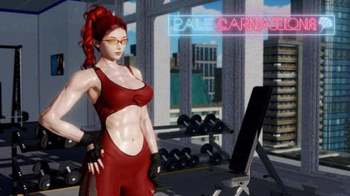
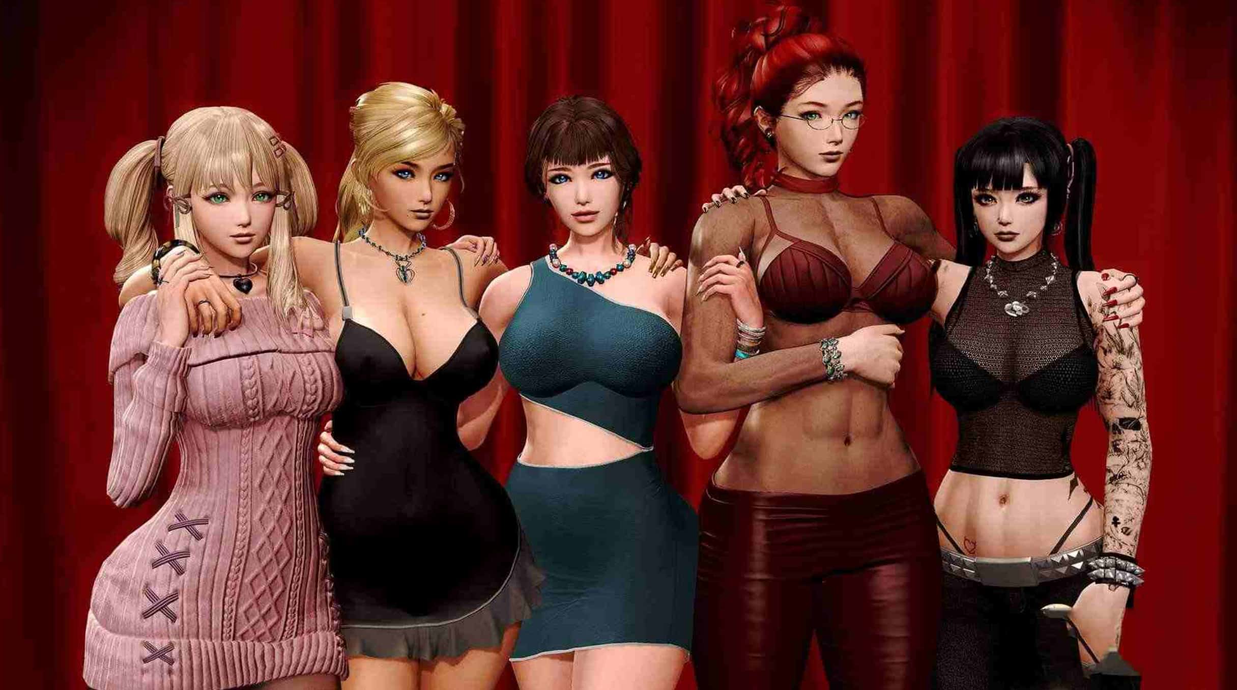
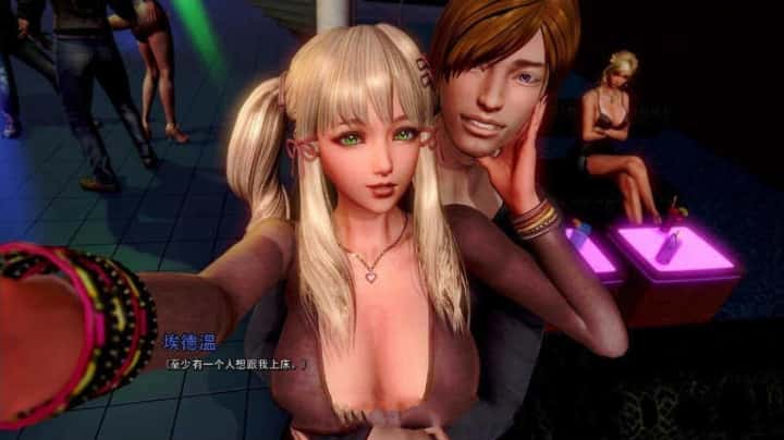
康乃馨俱乐部中的建模极其精美,女主角几乎都是超级大美女~ 游戏已经经过几次更新,内容非常丰富,而且有大量的动态CG! 目前出场的女主,有几个非常漂亮的都已经上垒了,剧情非常丰富! 剧情方面讲述了男主在一家高级私人会所工作的经历!
游戏特色
战斗系统
流畅的动作战斗体验
开放世界
自由探索广阔的游戏世界
多人合作
与朋友一起享受游戏乐趣
成就系统
丰富的挑战和奖励机制
游戏截图


游戏数据
⚡ 游戏秘籍
康乃馨俱乐部中,一位饱经创伤的医学预科学生走了进来。
这个学生虽然一心想过着简单的生活,但由于一个日渐堕落的儿时朋友的影响,他被吸引到了一个堕落的世界里。
作为康乃馨俱乐部的最新员工,在一系列残酷的情色游戏中为你的妹子指导。
你会放弃你的顾虑,被俱乐部的财富和充满**欲望的夜晚所诱惑吗?
或者在这一切结束的时候,一朵浪漫的爱情之花会发芽,迫使你把这它抛在脑后
为了摆脱给熊孩子当家教的生活,你踏入了这家俱乐部。
本游戏非单线剧情,所以回想全开需要反复读档,开头四个问题我选3>2>2>2,与他的热情相称>安抚>有限度的>称赞厨艺>谈论..>她的工作>说到..她的约会>告诉她这没什么>聊最近的电影>失陪去洗手间>短信选婉言拒绝(politely decline)>让伊恩说完>跟她调琴>短信选一切都很顺利(it went okay)>短信选我到了(I'm here)>跟他握手>赞美她的名字>我的好朋友<这里存档SAVE1>>告诉她可以加入>短信选我加入了(I'M in)>紧紧拥抱>用笑话感谢他>谢谢他>一直随便选>拿钱>选姓(表示尊重)>安抚>继续吧>看>这是什么意思>开玩笑>对她的工作表现出兴趣>这里存档save2>点费利西亚>左下返回>点米娜>点左下>点吧台>点酒保>一杯樱桃炸弹>点基友(基利安,人如其名...)>选第一个>点楼梯>选米娜(这里把我笑死...)>点费利西亚>我要再去看看米娜>点米娜>是啊,为什么不呢>点左下>舞池>米娜>告诉她真相(出卖基友...)>点左下>点米娜>帮帮米娜>叫他走开>挺身而出>让她知道这很酷>期待到来>你做的很好,放宽心>告诉她生日>吻她(解锁回想米娜01)>上演一出戏>我可不想.....>自己动手>接受费利西亚>迁就>要求一些隐私>我想>喉咙>告诉她(解锁回想费利西亚03)>问问他这是怎么回事>很抱歉让她久等>直接看>去你的!>短信选别担心(don't sweat it?)>向她呼喊>握手>说出事实>掏出来>选露西( 解锁回想MISC01,同维罗妮卡01,以后跟其他人物相同的就不说了)>请她喝咖啡>两个各选一次>告诉她她是对的>到底怎么回事?>我至少是好奇的>当然可以>谢谢你的建议(解锁回想MISC02)>问问维罗妮卡的事>转过身来>选后者(解锁回想维罗妮卡02)>维罗妮卡赢(解锁回想维罗妮卡03)>同意他的看法(解锁回想维罗妮卡04)>安抚地>现在太晚了,加倍>什么也不说>绝对没有(解锁回想MISC04)>很兴奋(解锁回想凯瑟琳04)>这里存档save3>跟着汉娜>当然>屁股>是在利用处于...>问问要不要进来坐坐,到目前终于解锁了所有菜单项,最重要的是STATISTICS,这里能查看每个人物的属性,非常重要!
断然否认>别耍...>夸全部(选这个加的属性最多)>选择前先存档SAVE4>罗莎林德合作>领队女孩?>问问她急什么>直接转向更...>告诉她拿出来>告诉她,他们没有错>随便选(解锁回想罗莎林德02)>同意帮汉娜>祝她们玩的开心>半真半假>同意陪米娜>直说你在想什么>毫不拘束的谈论裙子>告诉她这会给人留下深刻印象>看一下>继续看(不看白不看反正不减属性)>可爱路线>费利西亚>接受晚宴邀请>感谢米娜关心>把手放在>问问她怎么知道>告诉她用你的名字>说出感受>告诉接受交易(选这个是为了后面的一个ev)>随便选>还是随便选>问问她真的没问题吗>选第一个>里面>随便选(解锁回想罗莎林德03)>短信选第二个>告诉他你喜欢这里>谢谢他的好意>配合她>给我看更多(show me more)>讲个笑话>拉近>选鼻子>承认她的观点(解锁回想费利西亚06)>和老板打招呼>告诉他你值得信任>告诉哈娜他们很厉害>赞赏哈娜的纹身>说说哈娜的摩托车>钦佩她的坚韧>告诉她你只是在学习>算了吧,在泳池里玩的开心点>告诉凯瑟琳我已经准备这么做了>告诉凯瑟琳你真的不想>邀请米娜去健身房>告诉她你想变得更健康>通过道歉转移话题>寻求帮助>对他们坦诚相待>让她证明自己>取笑伊恩的童年>短信回你是好女孩(解锁回想罗莎林德04)
接下去就是俱乐部比赛了,这也是一个难点,能点的人都点一次>点左上逛>bar>点哈娜>告诉她你很抱歉...>能点的都点一遍(别忘记沙发上教授)>点左上逛>security>告诉沃伦这地方很有趣>左上逛>hallway>点汉娜或保安都可>保持专业>保持冷静的...>左上逛>更衣室>静静看着>摸摸......>告诉她不要自满(解锁回想维罗妮卡08)>左上逛>bar>能点的都点>左上逛>监控室>电脑>看一下>左上逛>VIP贵宾室>点中间>是的,继续>帮助维罗妮卡...>效仿凯瑟琳>谢谢她给我们这个机会>选择前先存档save5
接下去是重点,这里最快要打三次才能解锁全部回想,而每人必须赢一次,败一次,我的顺序是这样的:
第一次:冠军 罗莎林德 亚军 费利西亚 败 维罗妮卡
第二次:冠军 费利西亚 亚军 维罗妮卡 败 罗莎林德
第三次:冠军 维罗妮卡 亚军 罗莎林德 败 费利西亚
先来第一次,以后我们再通过读档来回收回想,喜欢温柔、顺从>感受到被关心的>告诉她,她做对了>用话语激励...>告诉继续>稍微戏弄下>告诉她还不够好>继续猛烈>告诉她你在尽最大努力表演>在脸颊(解锁回想费利西亚07)>是的站起来>饱受崇拜>要求她加快(解锁回想罗莎林德05)>确保她没事>拍拍她(解锁回想维罗妮卡09)>告诉基友别再做混蛋>两次最小功率(解锁回想维罗妮卡10)>选择前先存档save6>溜出去找哈娜
俱乐部比赛结束,是的,因为你有病态好奇心>我从来没用吸尘器...>我从来没有给同....(选这个解锁回想MISC06)>让女性拖延>我从来没有在约会时搭讪>吻她>告诉她你只在乎和她(解锁回想哈娜02)>愤怒的质问>自己的事情自己做>稍微超出(解锁回想维罗妮卡13)>热情的自我介绍>每张照片看一下>右上点继续>指那张全家福>随便选直到不谈论照片>逗她,你喜欢她的金发>盯着看>站起来强调>一只手...>转身赶人>坐在座位上身体前倾,看着>拖住下巴,看着眼睛>摸着“良心”说话>在说出下句台词的时候抓住...>加入自己的表演>米娜在等着呢,吻(解锁回想米娜04)>接受礼物>为了这个你想看哈珀的脸>非常详细的解释即将发生的事情>哈珀说是叔叔>上钩(解锁回想MISC07)>这是条件,现在照她说的做>随便选>带头扭转局面(解锁回想凯瑟琳10)
打电话给维罗尼卡>问问是不是一切都好>保持友好,像做生意一样>告诉她你只是在欣赏她背后>分享你的诚实想法>告诉她....>在其余的拍摄之前尝试温暖>使用亲密...>随便选>使用你自己的工具>别再让维罗尼卡不高兴>抓维罗尼卡>坚持让她做这项工作>武痴地...>选第一个>鼓励(解锁回想维罗妮卡14、15、16)>吻>告诉这么做是交易的一部分>先逗他>把这个带到隧道里>帮助唤醒她的记忆>吻>告诉她你不介意...>带着创造力和热情的配合>找一个新角度>尽可能长时间的抵制(解锁回想罗莎林德10、11、12)>睡在沙发(解锁回想哈娜03)>抱紧>强调钱的重要性(解锁回想哈娜04、05、MISC08)>说实话>(这里开始米娜属性已经很高了,所以怎么选问题都不大)试着温和地缓解她的担忧>拍拍她的头>问问她的工作情况>传达你在这个问题上的亲身经历>不要把注意力放在消极方面>逗她开心>告诉她她在工作中表现不错
接下去费利西亚剧情,一定要先跟费利西亚打招呼>拉近给个拥抱>讲个笑话>叫她深吸一口气>现在正是推动它的时候(解锁回想费利西亚12)>用它让她在拍照时偷偷...>跳到中等强度>与他的委托人和解是这位年轻经纪人的工作>转向费利西亚>继续,看看这会有什么结果>把它调到最大>挑战她>抓住费利西亚>实现她的梦想(这里选另一个的话会有此事件的另一个动态,可在回想里再去试)>取笑她>用不同的方式生火>享受更多(解锁回想费利西亚13、14、15)>提醒她,但你相信她能做到>(这里推荐存个档save7,因为这次选择影响到后续的剧情)选前两个会改变关系(被包),选第三个会提高双属性,但关系不变,我选的第三个>给基友打电话
大段剧情,告诉她维罗妮卡坚持要关闭健身房>点保安>去酒吧>点老板>你试着把它看做是工作>你宁愿得到别人的帮助>点达利亚>继续点达利亚>去监控室>去贵宾室>跟索菲亚说话>去更衣室>点基友那堆>告诉他罗莎林德的问题>好的你会向罗莎林德提出(一定要这么选,关系到后面的一个回想解锁)>点哈珀>去贵宾室>点教授>点阿尔伯>(这里存档SAVE8)罗莎琳>公平竞争>远程攻击>冲他下来,抓住他>猛按特殊按键.....>选第一个,摸头杀>越过这条线>接下去看着选吧(解锁回想米娜05)>亲下接受(米娜属性全满了,关系也是恋人)>让她按照自己的节奏来处理>给哈娜打电话
然后选项出来时存档SAVE9,现在先进行回想的回收工作,还有很多回想没开呢:
load:save1,占便宜>接下去看着选就行了(解锁回想罗莎林德01)
load:save2,点费利西亚>找酒保买一杯樱桃炸弹>回去找费利西亚>我看不出那有什么坏处>建议我们来一杯>我会表现出她的热情>莫奈子>使劲>这里看着选,有两个动态,可在回想里尝试(解锁回想费利西亚01)
load:save2,点费利西亚>找酒保买一杯樱桃炸弹>点基友>好计划>回去找费利西亚>我要再去看看米娜>点米娜>好啊,不过让我先邀请费利西亚>点费利西亚>去舞池点米娜>去吧台找基友帮忙>放开她!>期待着它的到来>你做的很好,让他们放松下>告诉生日>让她问费利西亚(解锁回想米娜01)>我不可能....>接受预付款>迁就>问问他想不想一起(解锁回想费利西亚04)
load:save3,这里比较麻烦,要重玩一大段剧情,开这个档是因为我的主线流程少了很多凯瑟琳的好感度以防万一,以后可以用这个档,帮普尔曼太太去她的办公室>主动提到外面去>比我想象的要享受的更多>第三局:维罗妮卡和你>接下去很多选项都是随意选,直到合作拍摄的时候,依然选罗莎林德就行>接着继续随便选直到5个选项出现的时候选234>拒绝汉娜party>祝他们玩的开心>然后一路CTRL一路随便选,碰到邀请都拒绝,直到出现敲门选项>等一会儿,先偷听(解锁回想凯瑟琳05)
load:save4
,与费利西亚合作>自己看着选就行(解锁回想费利西亚05)load:save4,与维罗妮卡合作>还是看着选就行(解锁回想维罗妮卡06)
load:save5,选第一个>再选第一个>告诉她,她做对了>闭嘴>等着她自己恢复>直接把放进等待的....>继续...>别理他>这可能会误会>是的,告诉她>饱受折磨>要求她加快>确保维罗妮卡没事>告诉她没问题>告诉基友做个好人(解锁回想罗莎林德06)>遥控两次都选低>留下来看>加入(解锁回想罗莎林德08)
load:save5,一个体贴的>虐待狂>告诉她,她做对了>闭嘴>等着她自己恢复>直接放进等待的....>继续....>别理他>那样会误会>是的,告诉她>受人崇拜>要求她加快>维罗妮卡这里选第二个>告诉基友做个好人(解锁回想费利西亚09
)>遥控两次都选低>留下来看>加入(解锁回想费利西亚10)load:save6
,留下来看(解锁回想维罗妮卡12)这样我们之前的回想也都回收完毕了,继续下面的剧情:
load:save9,
给予一些肯定>?????>展示你真实的一面>全力以赴(解锁回想罗莎林德14、15)>在俱乐部先点罗莎琳德>展示罗莎琳德的敏感性(解锁回想罗莎林德16)>点费利西亚那边>感到骄傲,把它拿出来(解锁回想费利西亚16)>点雅各布>利用你的地位帮助雅各布>点左上逛>BAR>先跟除了沙发上的哈珀一伙外的其他人对话一遍>然后点哈珀>过去打个招呼>让他谈谈自己和他一生的成功(解锁回想MISC09)>去奥古斯特房间找他聊天>去BAR找沙发上的聊天>去监控室找雅各布聊天得知摇滚乐室有状况>去摇滚乐室>让他们在欣赏的同时完成(解锁回想MISC10)>去泳池>去贵宾室>先和沙发上的聊天>再点吧台基友那边>采取更直接的方法让医生放过emma>去天鹅绒房>先点下除了凯瑟琳那一堆外的所有人>最后点凯瑟琳>到那边去>轻轻打一下不会有事>为观众上演一场美妙的演出(解锁回想维罗妮卡18)>试着安慰她>使用温和的方法>捏>采取感性的方法来获得答案>费利西亚可以接受这个>选第一个尝一尝(解锁回想费利西亚17)>好吧,如果你的匿名性得到保证>热情的问候....>主动发挥创造力>亲吻鼓励>保持冷静>选第一个(解锁回想罗莎林德17)> 存档save10
去拜访米娜>随便选(解锁回想米娜06)>对她坦诚>伊恩是个独立的个体>对你的朋友要坦率和诚实>修女听起来不错(nun sounds good)>随便选>忽略它,把你的注意力集中在Hana上>吻>抓住汉娜的手>采取更开放的方式>活在当下....(解锁回想哈娜07)>插话并打破紧张气氛>转移话题>随便选>把手放到....(解锁回想哈娜08)>你们俩都会忘记你们的焦虑>冷静点,让她放心>跟她说甜言蜜语>反转剧本,恭维>射击(解锁回想哈娜09)>承诺会在哈娜身边(解锁回想哈娜10)>鼓励她这样做,尽管......>这里存档SAVE11,因为关系到是成为女友还是纯粹玩伴
load save10:向凯瑟琳寻求建议>剧情过后解锁回想凯瑟琳14
load save11:我暂且选的第二个,玩伴,因为已经有了米娜>我喜欢你闻起来的味道(好像选别的没啥区别,反正好感是满的)>给自己电一下....>这里选全力以赴会减罗莎德林好感2,加凯瑟琳1,我选的全力以赴>别手下留情>这里选第一个会减费利西亚3点,加凯瑟琳1好感,2信任;选第二个会加费利西亚2好感,减凯瑟琳好感和信任,我选的第一个(解锁回想凯瑟琳15)>电普尔曼夫人>牵着她的手>腿>把她的手放回原来的位置>这里因为目前看不到索菲亚的数据,所以我还是选了第一个,能加凯瑟琳信任(解锁四个共通回想)>提到哈珀和露西>吻她的额头(重要提醒:这里关于米娜的一个未解回想08需要load save8,选择完罗莎林德后,在和mina和他弟弟游戏城结束后跟米娜到家里要选不越过线,且和哈娜不成为恋人就会触发,因为太长的剧情,我就不详细写了,反正这CG也没啥看点)>直接坦白>让她转过身去>随便选>加快>接下去都是随便选(解锁回想米娜09、misc15)>指责他>催促多说>这只是谨慎而已>给我看看>同意他.....>友好的.....>有一种吸引力是你无法否认的>存档save12>你有其他方式来度过你的不眠之夜>给哈娜打电话>你错过了她的声音>接下去都随便选(剧情后解锁回想哈娜11)
老妈剧情过后选有趣>打罗莎林德电话>打费利西亚电话>你是以她朋友的身份打电话>道歉>给维罗妮卡打电话>有可能的>存档save13>因为罗莎林德目前好感太低,且有个CG的时间点冲突,所以这边主线不选择和维罗妮卡去喝酒>问问罗莎林德还好吗>坚定立场>坐下>建议简单明了的解决问题>为罗莎林德做点好事>真的很高兴又有了一个室友>忽略你的想法(解锁回想罗莎林德23)>证明它>随便选(解锁回想哈娜12)>你还有成长的空间>提到阿尔伯前几天来过>这是我们的情报>同意坚持这种事情事错误的>抢在他之前行动(出现这段剧情的前提是之前按照我攻略做的让基友帮罗莎林德还钱)>直接说出名字>逗她开心>选第一个>你也很高兴重新....>和他击掌(解锁回想罗莎林德24)>热情的问候费利西亚>不要让她退缩>争取更多>我能请你喝一杯吗>把手放在她腰间>吻手礼>插嘴>背后安抚>谈论他们的历史>直率的取笑>要求(此时费利西亚的好感也满了)>想要出去玩的心理....> 存档save14>给她一点触摸>问问她最近怎么样>问问埃里克今晚对她好不好>你知道,但她不必担心>找个借口离开......>回到费利西亚那里>你的手不受控制的...>在那之前>警告她关于伟伦的事>假装她脸上有东西>建议她去找丹尼斯谈谈>存档save15>人越多越热闹(我主线走三人行线)>够了(解锁回想米娜10)
至此4.4的剧情就结束了,可以存档save16. 现在我们开始进行回想的回收工作:
load save12:你确实喜欢看>随便选(解锁回想MISC16)
load save13:今晚邀请她喝一杯>随便选一直到和维罗妮卡喝酒>跳舞?>告诉她她看起来也很漂亮>存档save17>放开所有顾虑,邀请跳舞(解锁回想维罗妮卡24)>你喝醉了,就坦诚相待吧>去做吧(解锁回想维罗妮卡25)>随便选>继续膜拜>随便选>你喜欢的>随便选(反正是走支线无所谓了)>随便选(解锁回想维罗妮卡26)
load save17:帮助维罗妮卡牵线搭桥>坚持赌约>大胆点.....>让她留下一会儿(解锁回想MISC17)>接下去一直随便选,直到见到费利西亚前(解锁回想维罗妮卡27)
load save14:给她一点触摸>问问她最近怎么样>问问埃里克今晚对她好不好>你知道,但她不必担心>找个借口离开......>一如既往,好奇心战胜了>省他麻烦,打招呼>随便选>你想弄清楚.....>建议她去找丹尼斯谈谈(与此同时你去找露西)>坦诚的向她表示....>呼吁同情心>让她靠近(解锁回想MISC18)
再次load save14:直接问她你的怀疑>告诉她今晚她看起来很好>问问哈珀和她还好吗>不幸的是,这是她要承担的风险>在你走之前,你必须多问一次>一如既往,好奇心战胜了>建议她去找丹尼斯谈谈(与此同时你去找露西)>玩弄恐惧>暗示你们应该有良好的关系>拉进距离并提醒>进一步推动(解锁回想misc19)
load save15:你真的只想和费利西亚单独>你不会再遇到.....>你是>随便选>感到浪漫(解锁费利西亚回想24)
好了,目前4.4的回想已经收集完毕,康乃馨的攻略真的不好做,花了我整整两晚时间,感觉我现在偏好更倾向费利西亚了(魅力无限),作者对于服装的设计和选择是真的很有品味啊!期待后面的剧情........